Start with a simple figure made up of a couple of parallel line segments.

Next, make a copy of the figure, shrink it, and arrange copies in an M-shape, flipping the middle copy vertically, and finally superimposing the copies on the original. (The M-shape comment will make sense in a minute.) The arrowheads aren’t part of the figure, just here to try to make the construction easier to follow.
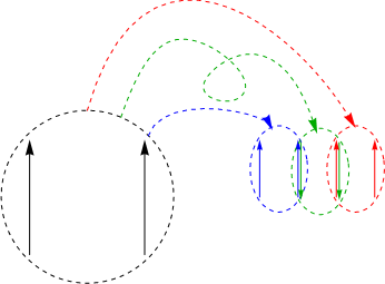
Superimposing the start figure with the scaled and rotated copies results in the first approximation to Hironaka’s curve.

Repeat the process of scaling, translating, and flipping.
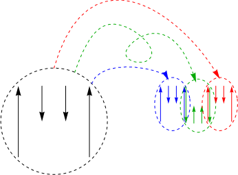
Superimposing all the pieces gives us the second approximation to Hironaka’s curve. The M-shape comment should make a little more sense now.
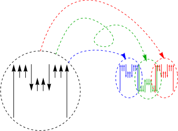
From the second iteration to the third:
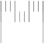
Do this enough times, and you’re approximating Hironaka’s curve, sometimes called Hironaka’s M-curve.
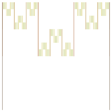
The individual pieces look like this, which are interesting enough in a Cantor set kind of way:

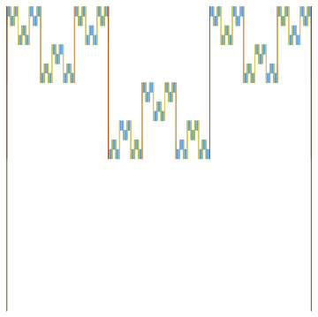
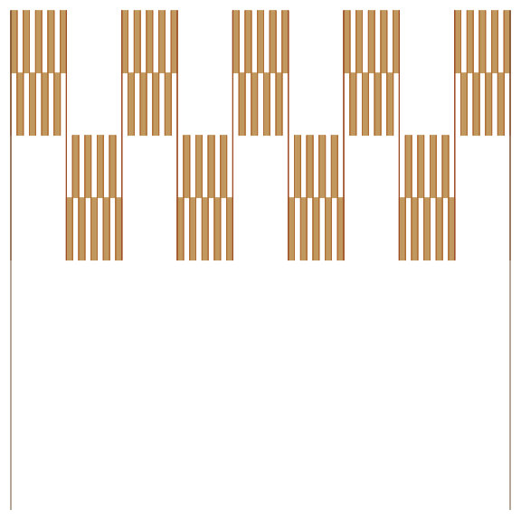
The figure can be generalized for different numbers of copies made at each step, in this case five:
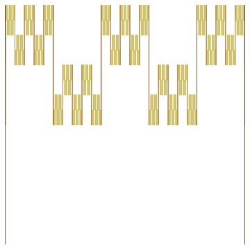
Or seven:
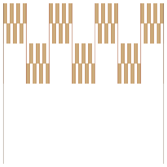
Or nine:
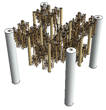
It can also be generalized to 3-D, though not very legibly:
If you’re interested, the Mathematica code for the first figures:
Hironaka[0] = {Line[{{0, 0}, {0, 1}}], Line[{{1, 0}, {1, 1}}]};


Hironaka[n_] :=

 Hironaka[n] =

  {Translate[Scale[Hironaka[n - 1], {1/3,  1/2}, {0, 0}], {0/3, 1/2}],

   Translate[Scale[Hironaka[n - 1], {1/3, -1/2}, {0, 0}], {1/3, 2/2}],

   Translate[Scale[Hironaka[n - 1], {1/3,  1/2}, {0, 0}], {2/3, 1/2}]}


Graphics[{Thin,

  Table[{ColorData["SouthwestColors"][i/5], Hironaka[i]}, {i, 5, 0, -1}]}]
The others follow similarly.
See Gerald A. Edgar, Measure, Topology, and Fractal Geometry, Springer-Verlag, 1990, pp. 203–204.
See also Curtis McMullen’s https://people.math.harvard.edu/~ctm/gallery/ and
https://people.math.harvard.edu/~ctm/gallery/cx/Mcurve.gif.
Thanks to Roger Bagula for the generalization idea.
Figures created with Mathematica 10.
Robert Dickau, 2016.
[ home ] || [ 2016-06-14 ]
robertdickau.com/hironaka.html