L-systems (also called Lindenmayer systems or parallel string-rewrite systems) are a compact way to describe iterative graphics using a turtle analogy, similar to that used by the LOGO programming language. An L-system is created by starting with an axiom, such as a line segment, and one or more production rules, which are statements such as “replace every line segment with a left turn, a line segment, a right turn, another segment...”. When this system is iterated several times, the result is often a complicated fractal curve.
When programming L-systems, one typically represents the axiom as a sequence of
characters, such as F, and the production rules as replacement rules of the
form F -> F+F--F+F. We then carry out the string replacements (in parallel)
as many times as desired. For example, we iterate the axiom and production rule just
described in the following way:
We start with the axiom F, and replace every occurrence of F with
F+F--F+F, resulting in the string
F+F--F+F.
We then replace every occurrence of F in the result with F+F--F+F,
resulting in the string
F+F--F+F+F+F--F+F--F+F--F+F+F+F--F+F.
Carrying out the replacement one more time results in the following:
F+F--F+F+F+F--F+F--F+F--F+F+F+F--F+F+F+F--F+F+F+F--F+F--F+F--F+F+F+F--F+F--
F+F--F+F+F+F--F+F--F+F--F+F+F+F--F+F+F+F--F+F+F+F--F+F--F+F--F+F+F+F--F+F
.
After the desired number of iterations has been carried out, we render the L-system
string using the turtle analogy. A typical interpretation of our string is that an
F is an instruction to draw a line segment one unit in the current direction,
a + is an instruction to rotate the current direction one angular unit clockwise, and
a - is an instruction to rotate the current direction one angular unit
counterclockwise. (Other characters and interpretations are of course up to us.)
If we assume for this example that one (angular) unit is π/3 radians, the
following are the partial results (omitting the zeroth iteration, the axiom).
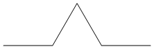
First iteration (F+F--F+F):
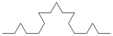
Second iteration (F+F--F+F+F+F--F+F--F+F--F+F+F+F--F+F):
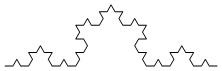
Third (F+F--F+F+F+F--F+F...(148 characters in all)...F+F+F+F--F+F):
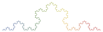
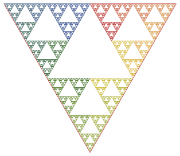
In the following pictures, the rendered L-systems are colored using the progression red-orange-yellow-green-blue-purple-red from beginning to end, to better illustrate the “path” of the curves.
(Axioms, production rules, and Mathematica code are below the pictures. These ideas can also be extended to three dimensions.)
Koch curve (F -> F+F--F+F, 60°):
32-segment curve
(F -> -F+F-F-F+F+FF-F+F+FF+F-F-FF+FF-FF+F+F-FF-F-F+FF-F-F+F+F-F+):
Hilbert curve (L -> +RF-LFL-FR+, R -> -LF+RFR+FL-):
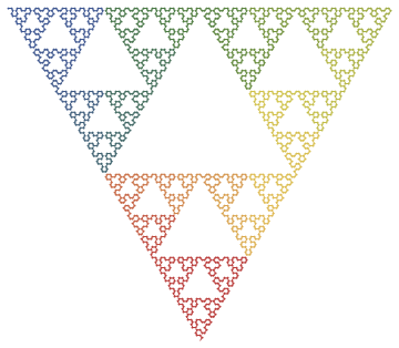
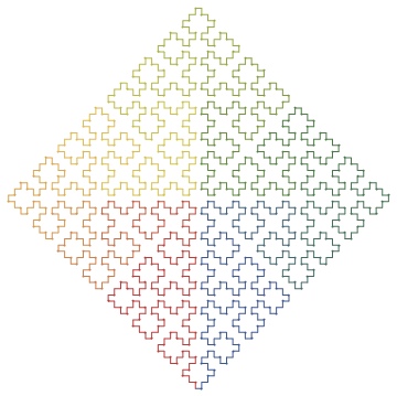
Arrowhead curve (X -> YF+XF+Y, Y -> XF-YF-X, 60°):
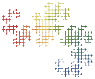
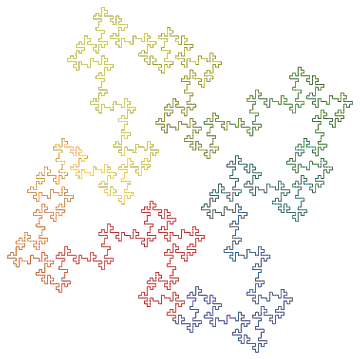
Dragon curve (X -> X+YF+, Y -> -FX-Y):
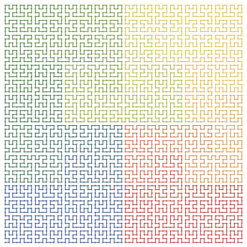
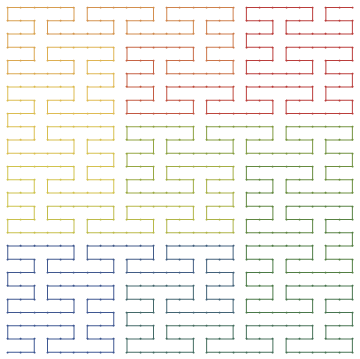
Hilbert curve II (X -> XFYFX+F+YFXFY-F-XFYFX,
Y -> YFXFY-F-XFYFX+F+YFXFY):
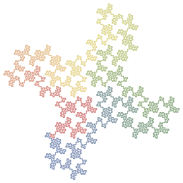
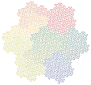
Peano-Gosper curve (X -> X+YF++YF-FX--FXFX-YF+,
Y -> -FX+YFYF++YF+FX--FX-Y, 60°):
Peano curve (F -> F+F-F-F-F+F+F+F-F):

Quadratic Koch island (F -> F-F+F+FFF-F-F+F):
Square curve (X -> XF-F+F-XF+F+XF-F+F-X):
Sierpinski triangle (F -> FF,
X -> --FXF++FXF++FXF--, 60°):
Here’s the embarrassing old-school code (the functions
LShow and LShowColor are identical except that LShow
displays the system using only a black line, works a bit faster, and takes less
memory):
(* carry out the forward and backward moves and the various
    rotations by updating the global location 'Lpos' and
    direction angle 'Ltheta'. *)

Lmove[ z_String, Ldelta_ ] :=
    Switch[ z,
        "+", Ltheta += Ldelta;,
        "-", Ltheta -= Ldelta;,
        "F", Lpos += {Cos[Ltheta], Sin[Ltheta]},
        "B", Lpos -= {Cos[Ltheta], Sin[Ltheta]},
         _ , Lpos += 0. ];

LSystem::usage =
    "LSystem[axiom, {rules}, n, Ldelta:90 Degree]
    creates the L-string for the nth iteration of
    the list 'rules', starting with the string 'axiom'.";

(* make the string: starting with 'axiom', use StringReplace the
    specified number of times *)

LSystem[ axiom_, rules_List,
    n_Integer, Ldelta_:N[90 Degree] ] :=

    Nest[ StringReplace[#, rules]&, axiom, n ];

Off[General::spell1];

(* initialize the position 'Lpos' and the direction angle 'Ltheta';
    create the Line graphics primitive represented by the L-system by
    mapping 'Lmove' over the characters in the L-string, deleting all the
    Nulls; then show the Graphics object *)

LShow[lstring_String, Ldelta_:N[90 Degree]] :=
   (Lpos={0.,0.};
    Ltheta=0.;
    Show[
      Graphics[Line[
        Prepend[
          DeleteCases[
            Map[Lmove[#, Ldelta]&, Characters[lstring]],
           Null ],
        {0,0}]]],
     AspectRatio -> Automatic]);

(* same as above, plus a list of colors for each segment contained in
    'templist' -- unfortunately, 'templist' isn't really 'temp', but
    stays in memory as a global variable; so sue me *)

LShowColor[lstring_String, Ldelta_:N[90 Degree]] :=
   (Lpos = {0., 0.};
    Ltheta = 0.;

    templist =
      Map[ Line,
        Partition[
          Prepend[
            DeleteCases[
              Map[ Lmove[#, Ldelta]&, Characters[lstring] ],
             Null],
           {0,0}],
         2,1]];

    ncol = N[Length[templist]];

    huelist = Table[ Hue[k/ncol], {k, 1., ncol} ];

    Show[
      Graphics[
        N[Flatten[Transpose[{huelist, templist}]]]],
     AspectRatio -> Automatic]);

On[General::spell1];

LShowColor[ (* Koch curve *)
    LSystem["F", {"F" -> "F+F--F+F"}, 4],
        N[60 Degree]]

LShowColor[ (* Peano curve *)
    LSystem["F", {"F" -> "F+F-F-F-F+F+F+F-F"}, 4]]

LShowColor[ (* Quadratic Koch island *)
    LSystem["F+F+F+F", {"F" -> "F-F+F+FFF-F-F+F"}, 3]]

LShowColor[ (* 32-segment curve *)
    LSystem["F+F+F+F",
    {"F" ->
     "-F+F-F-F+F+FF-F+F+FF+F-F-FF+FF-FF+F+F-FF-F-F+FF-F-F+F+F-F+"},
    2]]

LShowColor[
    LSystem["YF", (* Sierpinski arrowhead *)
     {"X" -> "YF+XF+Y", "Y" -> "XF-YF-X"}, 7],
        N[60 Degree]]

LShowColor[ (* Peano-Gosper curve *)
    LSystem["FX",
      {"X" -> "X+YF++YF-FX--FXFX-YF+",
       "Y" -> "-FX+YFYF++YF+FX--FX-Y"}, 4],
     N[60 Degree]]

LShowColor[ (* Sierpinski triangle *)
    LSystem["FXF--FF--FF",
    {"F" -> "FF",
     "X"->"--FXF++FXF++FXF--"}, 6], N[60 Degree]]

LShowColor@LSystem["F+XF+F+XF", (* Square curve *)
    {"X"->"XF-F+F-XF+F+XF-F+F-X"}, 4]

LShowColor[ (* Dragon curve *)
    LSystem["FX", {"X"->"X+YF+", "Y"->"-FX-Y"}, 12]]

LShowColor@LSystem["L", (* Hilbert curve *)
    {"L" -> "+RF-LFL-FR+", "R" -> "-LF+RFR+FL-"}, 6]

LShowColor@LSystem["X", (* Hilbert curve II *)
    {"X" -> "XFYFX+F+YFXFY-F-XFYFX",
     "Y" -> "YFXFY-F-XFYFX+F+YFXFY"}, 3]
Designed and rendered using Mathematica versions 2.2 and 3.0 for the Apple Macintosh.
See also Peitgen et al, Chaos and Fractals, Springer-Verlag, 1992; Stan Wagon, Mathematica in Action, W. H. Freeman and Co., 1991; and Roger T. Stevens, Fractal Programming in C, M&T Books, 1989.
© 1996–2026 by Robert Dickau
[ home ] || [ 97???? ]
www.robertdickau.com/lsys2d.html